migraDASH

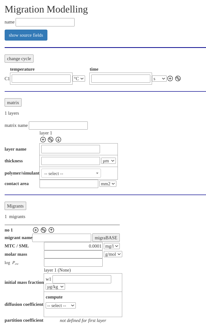
overviews of the full modelling form

migraDASH is our graphical user interface to the migration modelling service migraSIM. There are different views for the input of the migration modelling (depending on your permissions) and a dashboard for the results. If you need another/special view please contact us. In the following the full modelling form is discussed. The full modelling form is our most flexible view, a screen shot is on the right side.

The form start with a section, where you can load/store a configuration, i. e. a simulation describtion or load a template of a migration modelling scenario, the extended KTW cold water test temperature/time profile for example. After this a section where you can describe you project follows. This description will be added to the PDF report you can download from the results.

The main part of the form is the information needed for the migration modelling simulation and is devided into three parts:

for the time and temperature conditions
for the description of the polymer and food simulant/water layers.
for the description of on or more migrants containd in the polymer (oder simulant) layers.

If you click on , or you can hide/show the section.

You can specify your on data, or choose predefined polymer and food simulants or water in migraDASH. Also you can lookup the migrants information related to migration from our database migraBASE.

symbol	meaning
	add a change cycle, layer or migrant after the current
	copy a change cycle, layer or migrant
	remove a change cycle, layer or migrant
	show more information (needed by "user defined")
	show less information

Detailed Description of the form

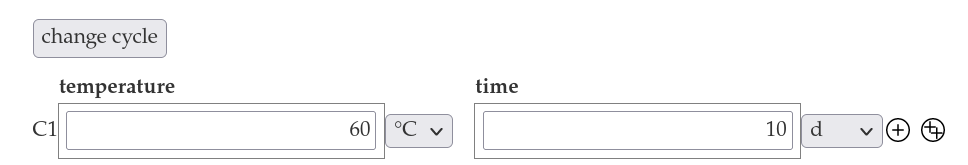
Temperature/Time cycles section

You can specify a temperature/time profile of consecutive cycles, with each cycle can have a different temperature and time period. With the , or buttons you can add, copy or remove a cycle. The cycles are numbered at the left with the suffix 'C'. You can use multiple cycles to model repeated use or time/temperature profiles, which are not constant over the time.

Modes

The of the cycle discribes the kind of the simulation during this period. Possible values are:

migration (default)
set off

Migration

During the mode migration the migrant moves from in the matrix according to the Fick's law of diffusion and the partitioning.

Set off

During the mode set off, the migrant moves in all the layers with contact (i. e. all layers with an initial mass fraction different from 'no contact'). The layers are assumed, to be on a roll, i. e. there is contact between the most left layer and the most right layer.

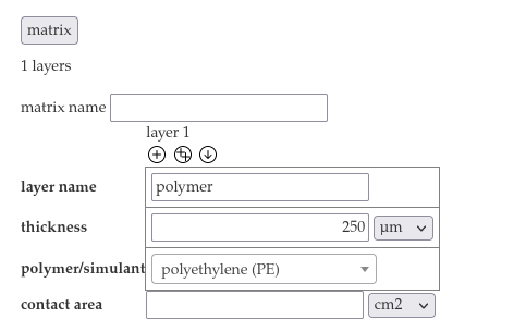
Matrix section

In the matrix section you specify one or more layers of the matrix, i. e. the polymers and the food simulant or water. With the , or buttons you can add, copy or remove a layer. For each layer you need to put in:

a name of the layer, the name must be unique for each layer.
a thickness or the volume of the layer
which polymer/simulant

Additionally the contact area needs to be specified. You can choose the polymer/simulant form a predefined list of around 140 polymers and 5 simulants. Alternativelly you can put user defined values for the polymer. Choose the button and insert the density. For the determination of the diffusion coefficients with the Piringer method (recomended) the \(A_p'\) and \(\tau\) value is needed. Details of the Piringer method you found in the fundamentals and the references herein. If the \(A_p'\) and \(\tau\) value is not available, it can be estimated with the glass transition temperature. Insert the glass transition temperature an choose "glass transition temperature" for the "compute" drop down menu in the Piringer section.

Migrant section

You can specify several migrants for each simulation. With the , or buttons you can add, copy or remove a migrant. With the button you can hide the details of the migrant, with the button you can show it agian.

For each migrant you need to specify:

a name of the migrant
the molar mass of the migrant
the logarithm of the octanol/water partition coefficient \(\log P_{ow}\)
the initial mass fraction in each layer
the diffusion coefficient in each layer
the partition coefficient in each layer

Molar mass and \(\log P_{ow}\)

You can enter the CAS number to the name field an click "migraBASE" to automatically lookup the molar mass and the \(\log P_{ow}\). Otherwise you can add the numbers manually.

Initial mass fraction

You need to specify the initial mass fraction for the first cycle in each layer. The migration will be homogenously distributed in the layer. If you specify the initial mass fraction for any futher cycle, the initial mass fraction will be set at the beginning of this cycle to the specified value, homogenously distributed. For example if this is used in the simulant layer a repeated use can be simulated.

If you not specify the initial mass fraction for any cycle after the first, the simulation will continue with the next cycle without changing the computed value, i. e. the value is kept. This is the default behaviour if the value is empty or if the option "keep" is explicitly selected. If you choose "no contact", this layer take no place in the migration for this cycle. For example a storage period can be simulated.

The initial mass fraction for the cycle 'Cn' is numbered with 'wn'.

Diffusion coefficient

The diffusion coefficient can be set to a user defined value, or it can be estimated with the Piringer or Welle approach. For the estimation with the Piringer approach the \(A_p'\) and \(\tau\) must be set for this layer in the matrix.

If user defined values are used, than for each cycle 'Cn' a diffusion coefficient 'Dn' can be specified. If the diffusion coefficient is not specified for each cycle, then the diffusion coefficient for the last specified cycle holds for all the following cycles.

Partition coefficient

The partition coefficient can be set to a user defined value, or it can be estimated with the \(\log P_{ow}\). This estimation is only used between a polymer and a food simulant or between a polymer and water. Between two polymer layers the partition coefficient is set to \(1 \frac{\text{mg/l}}{\text{mg/l}}\) if you choose \(\log P_{ow}\).

If user defined values are used, than for each cycle 'Cn' a partition coefficient 'Pn' can be specified. If the partition coefficient is not specified for each cycle, then the partition coefficient for the last specified cycle holds for all the following cycles.

Starting a simulation

If you have finished the specification of your scenario, you can submitt your form with the -button. A new window will popup (check if you browser allows popup windows) with a dashboard with the results.

Dashboard with the results

The new window shows the result of the migration simulation.

result

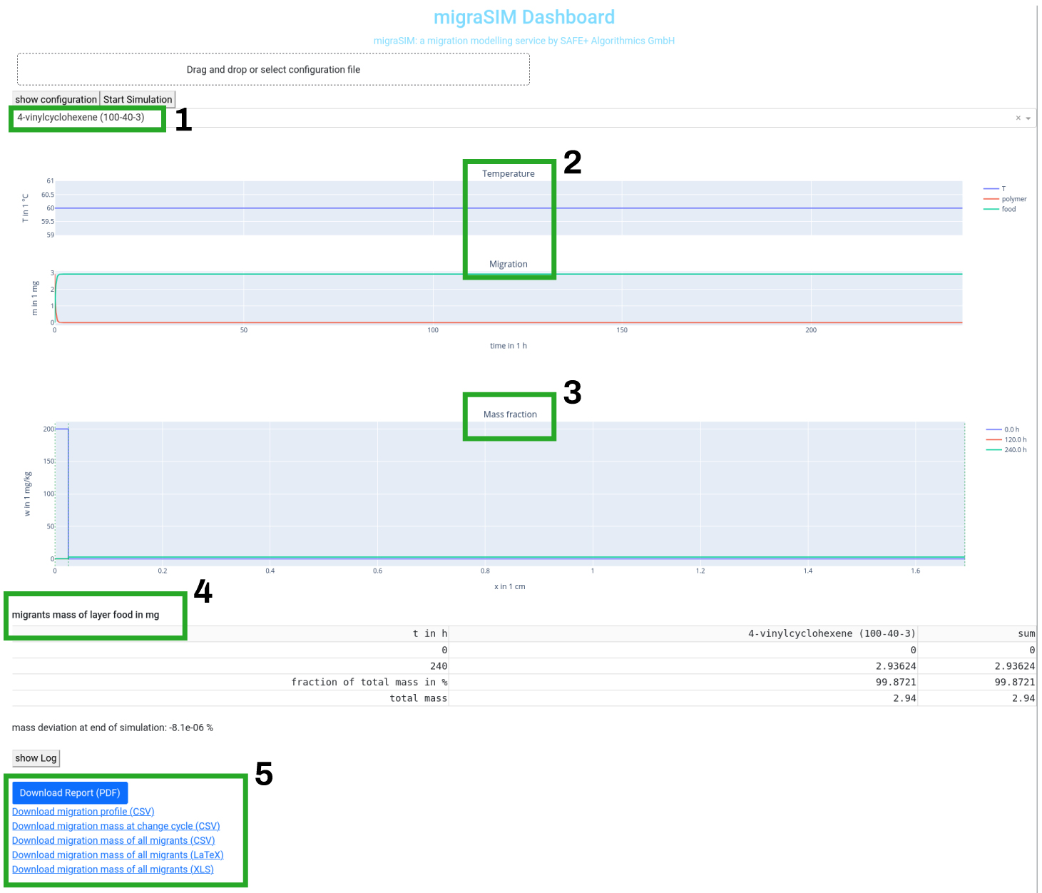
The drop down menu selects the migrant [1], for which the results are shown.

Migration profile [2]

The first graph shows in its upper part the temperature profile and in the lower part the migration profile in each layer for the choosen migrant.

If the mouse if moved to the right upper corner of the graph, icons for naviation/zooming and saving the graph appears.

Mass fraction profile [3]

The second graph shows the mass fraction profile over the matrix for the choose migrant for the initial state, the middle of the simulation and the end of the simulation. Each border between the layers is marked with a green dahsed line.

If the mouse if moved to the right upper corner of the graph, icons for naviation/zooming and saving the graph appears.

Table migrants mass [4]

The table migrants mass gives a short overview of all the migrants for the last layer (typically the food simulant or drinking water layer) and for the sum of all migrants. It shows the mass in the layer a the beginning and at the end of the simulation. It also shows the fraction of the total mass of the migrant, which is migrated into to last layer and finial it shows the total mass of the migrant. This means the total migration can easily derived from this last line of the table.

Saving results as tables or a report [5]

At the end of the results, there are links to tables as comma separated files, excel files or a PDF report for saving the migration simulation for documentation or post processing.

, click here to download a report as PDF file. The report includes the user input of the migration modelling, the used parameter from migraBASE and the results of the migration simulation. The geneation of the report takes some time.

You can use the following links to download the results in a file format, which can be post processed.

Download migration profile (csv)
Download migration mass at change cycles (csv)
Download migartion mass of all migrants (csv)
Download migartion mass of all migrants (LaTeX)
Download migartion mass of all migrants (XLS)

Tutorial: full modelling form, monolayer polymer

In this short tutorial a migration simulation will be done step-by-step for the migrant 4-vinylcyclohexene (CAS 100-40-3) from a monolayer polymer into olive oil.

Go to out site https://service.saferithm.com and the stage "production" or "testing" for migraDASH
Login in with you credentials.
Click on the "full modelling form".
Insert the temperature 60 and the time 10 days into as the change cylce.
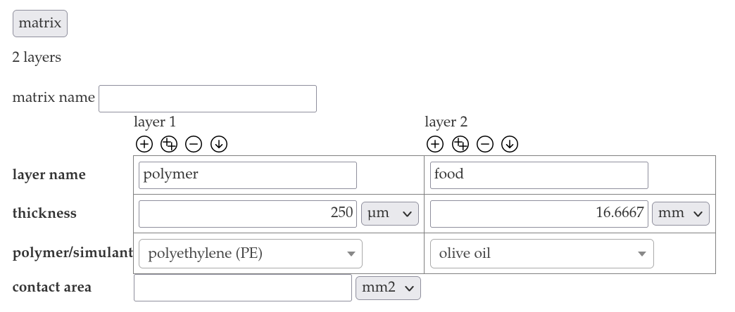
Choose "polyethylene (PE)" as the polymer and insert a layer name "polymer" and the thickness 250 µm into the matrix section.
Add a second layer with the -Button.
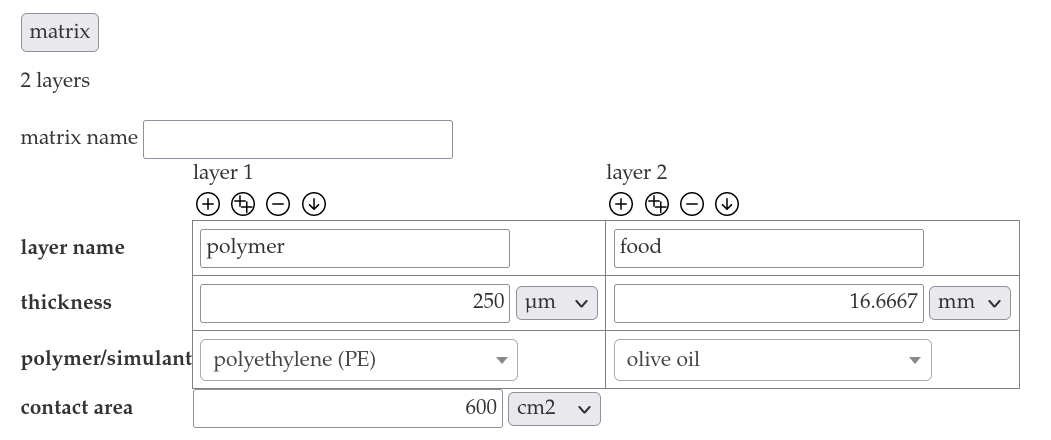
Choose "olive oil" from the dropdown menu of layer 2 and insert the layer name "food" the the thickness 16.6667 mm
Add the contact area 600 cm².
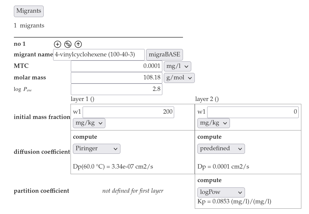
Insert the cas number 100-40-3 into the migrant name in the migrant section an click on "migraBASE". 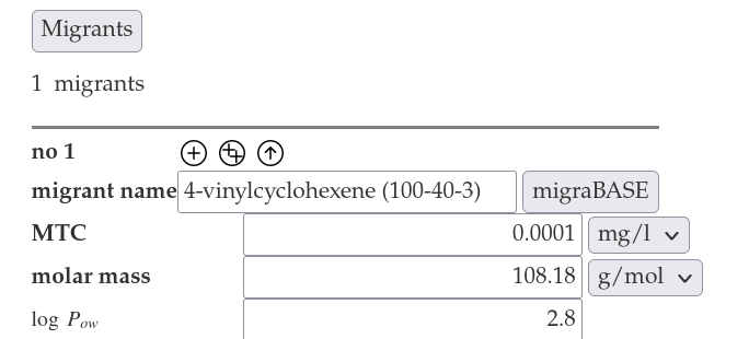This will lookup the cas number in the migraBASE database an fill in the molar mass and the log Pow.
Insert the initial mass fraction 200 mg/kg for the polymer layer, ant select Piringer for the computation of the diffusion coefficient.
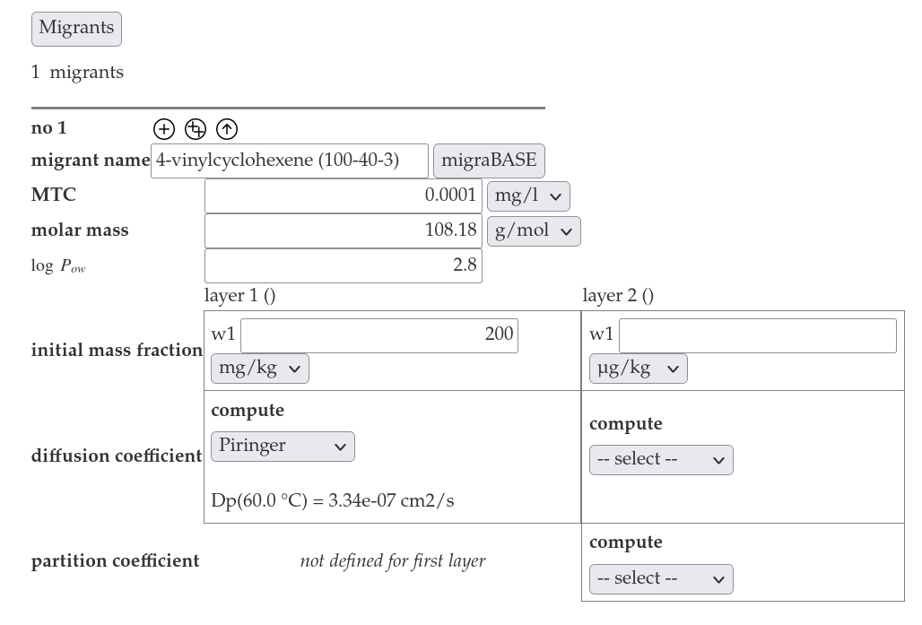
Insert "0 mg/kg" for the initial mass fraction for the food layer and select predefined for the computatio of the diffusion coefficient. Select logPow for the computation of the partition coefficient.
Press the "Submit"-button. In a new window the result of the simulation will be shown.
You can view the migration profile and the mass fraction profile in two graphs.
Press the -button and wait for the preparation of the report and the start of the download of the PDF-file.